DriftWorld: an action-conditioned world model based on drifting generative models. Generates future frames from the current observation and a candidate action sequence in a single forward pass at 30+ fps (17x faster than diffusion-based baselines).

Summary

The world model is conditioned on $c = (o_{t-F:t}, a_{t: t+T})$ where:

• $o_{t-F:t}$ = initial/current observation plus any history frames
• $a_{t: t+T}$ = proposed sequence of future robot actions
• $x = o_{t+1:t+T+1}$ = the future video the model should generate So the desired conditional distribution is: $$p(x \mid c) = p(o_{t+1: t+ T + 1} \mid o_{t-F:t}, a_{t: t+T})$$The generator produces: $x_i = f_\theta(\epsilon_i, c), \epsilon_i \sim p_\epsilon$, giving a model distribution: $$q_\theta(x \mid c)$$

• Conditional drifting field defined by the initial observation and action sequence, with a modification that accentuates action following (bias against $\hat{o}_{t+1} \approx o_t$)

  • i.e., for each specific starting scene and proposed robot action sequence, build a sector vector field that tells generated future videos how to move toward the correct feature, & modify that field so predictions that merely copy the starting frame are pushed away more strongly
  • 🔑 Conditional - means that samples are only compared within the same starting observation and action sequence
    • ^ a batch containing $B$ different demonstrations therefore has $B$ separate drifting fields, rather than one global field mixing unrelated scenes and actions.

• A drifting feature space that leverages DINOv2/v3 to maintain visual sharpness in complex scenes

• A U-Net architecture that ensures each video frame is precisely conditioned on the corresponding action

Training: $$\boxed{\text{noise + history + actions} \rightarrow \text{U-Net} \rightarrow \text{future VAE latents} \rightarrow \begin{cases} \text{VAE latent drift loss}\\ \text{decode} \rightarrow \text{DINO drift loss} \end{cases}}$$Inference:$$\boxed{\text{noise + history + actions} \rightarrow \text{U-Net} \rightarrow \text{future VAE latents} \rightarrow \text{VAE decoder} \rightarrow \text{future images}}$$

A note on indexing

As a note, the paper has a notational inconsistency: in Section 3.1 it writes actions $$a_{t:t+T} = (a_t, \ldots, a_{t+T})$$which contains $T+ 1$ actions, and predicts $$o_{t+1: t+ T+ 1}$$which contains $T+1$ future frames. But Algorithm 1 uses: $$\text{action shape } [T, D], \quad \text{positive video shape } [1, T, C, H, W]$$which implies $T$ actions with $T$ future frames, i.e. - $$(a_t, \ldots, a_{t+T - 1}) \rightarrow (o_{t+1}, \ldots , o_{t+T})$$ None of this impacts the core ideas presented, and these notes also may have inherited some of the notational inconsistency (I tried to stick with $(a_t, \ldots, a_{t+T}) \rightarrow (o_{t+1}, \ldots , o_{t+1+T})$, but some parts may be off by one) - please ignore any inconsistencies!

Drifting field

Vanilla conditional drifting field

For one condition $c$, let:

• $y^+$ = the real ground-truth future video for that condition
• $y_1^-, \ldots, y_N^-$ = generated future videos under the same condition

The drift acting on generated sample $x_i$ is (intuitively): $$V_{p, q_\theta}(x_i \mid c) = V_p^+ (x_i \mid c) - V_{q_\theta}^- (x_i \mid c)$$The positive term attracts $x_i$ to the real future (minimizing $\mathcal{L}$ will minimize $V$ which minimizes $V^+$, i.e. vector difference between $y^+$ and $x_i$) while the negative term accounts for nearby generated samples (minimizing $\mathcal{L}$ will maximize $V^-$, i.e. prevent generated samples from collapsing to one spot): $$V_p^+(x_i \mid c) \approx w_i^+ (y^+ - x_i), \quad V_{q_\theta}^- (x_i \mid c) \approx \sum_{j\neq i} w_{ij}^- (y_j^- - x_i)$$The weights are based on similarity, through some kernel $K$: $$w_i \propto K(x_i, y^+), \quad w_{ij}^- \propto K(x_i, y_j^-)$$The update target is: $$x_i^\text{drift} = x_i + V_{p, q_\theta}(x_i \mid c)$$The training loss is: $$\boxed{\mathcal{L}_\text{drift} = \mathbb{E}_\epsilon \left[||f_\theta(\epsilon, c) - \text{stopgrad} (f_\theta(\epsilon, c) + V_{p, q_\theta}(f_\theta(\epsilon, c) \mid c))||^2_2\right]}$$

• 💡 So the network output is trained to move in the direction prescribed by the field!

Adding the no-action future to the negative distribution

A common failure mode is the world model ignoring the action and simply copying the current image: $$\hat{o}_{t+1} \approx o_t$$This still achieves a deceptively low reconstruction error because most pixels (the table, walls, background, stationary objects) do not move. To prevent the model from falling in this trap, DriftWorld adds the no-action-future to the negative distribution (i.e. vector field of things to not do):$$\underbrace{\tilde{q} (x \mid a_{t: t+ T}, o_{t-F:t})}_\text{model's generated-future distr.} = (1 - \gamma) \underbrace{q_\theta(x \mid a_{t: t+T}, o_{t-F:t})}_\text{current distr. of model generated futures} + \gamma \underbrace{p(x \mid \varnothing , o_{t-F:t})}_\text{distr. corresponding to taking no action}$$where $\gamma \in [0, 1)$. Dissecting this equation in more detail:

• $q_\theta(x \mid a, o)$ is the model's generated-future distribution
• $p(x \mid \varnothing, o)$ is the distribution corresponding to taking no action
• In practice, the current frame $o_t$ is used as a real no-action negative - i.e. the unchanged current image is treated as an example of what the future should not look like when a nonzero action is commanded
  • Algorithm 1 (paper) writes this as: $$\texttt{yneg} = \text{cat}([x, \text{obs}[-1]]),$$where $x$ = $N$ generated future samples, $\text{obs}[-1] = o_t$ = most recent real observation.
    • 📍 Slight nuance: for the real-world datasets, the model predicts 1 future frame per call (and then autoregressively generates), so $o_t$ naturally has the same shape as the generated future. For a multi-frame output, one would need to construct a matching no-action chunk, e.g. by repeating $o_t$, but the paper's pseudocode does not spell out this case.
  • 🔑 So the negative set is: $$\mathcal{N} = \{x_1, \ldots, x_N, o_t \}$$
• $\gamma$ controls how strongly the model is discouraged from simply preserving the current state

The modified field is therefore: $$V_{p, \tilde{q}}(x \mid c) = V_p^+ (x \mid c) - V_{\tilde{q}}^-(x \mid c )$$where the negative part is conceptually: $$\boxed{V_{\tilde{q}}^- \approx (1-\gamma)V_{q_\theta}^- + \gamma V_{\text{no-action}}^-}$$The extra term $-\gamma V_\text{no-action}^-$ pushes generated videos away from futures that look like "nothing happened."

Drifting feature space

DriftWorld measures attraction & repulsion between particles via feature-space, rather than RGB space / raw particle (in this drifting field, images) space.

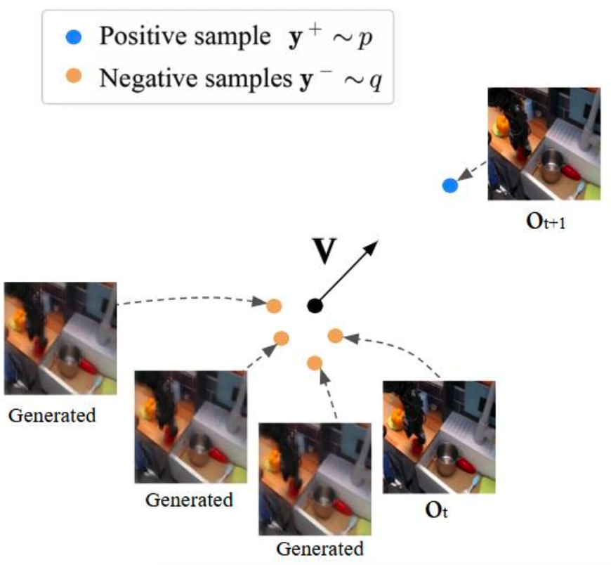
Particles in DriftWorld's drifting field

The particles are the model's generated future-video samples.

For one fixed condition $c = (o_{t-F: t}, a_{t: t+ T})$, the model samples different Gaussian noises $\epsilon_i \sim \mathcal{N}(0, I), \,\, i \in [1, N]$, and each noise produces one generated future chunk: $$x_i = f_\theta(\epsilon_i, c) \implies \boxed{\text{one particle }x_i = \text{one generated candidate future video}}$$For $T = 1$, a particle is one predicted next frame. For $T>1$, a particle is an entire predicted future chunk: $$x_i = \left(\hat{o}_{t+1}^{(i)}, \ldots, \hat{o}_{t+1+T}^{(i)}\right)$$

• 🔑 The model generates multiple particles under the same history and actions because different Gaussian noises $\epsilon_i$ may represent different plausible futures.
• 🔖 Bookkeeping: For one training example, we have...
  • one positive future $y^+$
  • $N_\text{neg}$ generated particles $x_1, \ldots, x_{N_\text{neg}}$
  • optionally the no-action image $o_t$ as an additional negative
• 📍 The paper's reported numbers of generated negatives are:
  • Push-T: $N_\text{neg} = 8$
  • Robomimic: $N_\text{neg} = 32$
  • Bridge-V2/RT-1/Language Table: $N_\text{neg} = 64$
• Sneak peek at content of following sections: Each generated particle $x_i$ receives its own drift vector $V_i = V_{p,q}(x_i)$. The target for that particle is $$x_i^\text{target} = \text{stopgrad}(x_i + V_i)$$

Feature space drifting

1. Pass each image through a frozen visual encoder $\phi$: $$\phi: \mathbb{R}^{C \times H_0 \times W_0}\rightarrow \mathbb{R}^{H \times W \times D}$$where $C$ = number of image channels (usually $C = 3$ for RGB), $H_0$ = original image height in pixels, $W_0$ = original image width in pixels. DINO transforms the image into a lower resolution grid: $H$ = number of feature-grid rows, $W$ = number of feature-grid columns, $D$ = number of features stored at each grid location. For DINOv3 feature vectors: at each location $(h, w) \in [0:16, 0:16]$, we have a 768-dim. feature vector describing the corresponding image region: $$\phi(x)_{h,w} \in \mathbb{R}^{768}$$
   • For real-world datasets, $\phi$ is DINOv2 or DINOv3.
   • After passing an image $x$ through $\phi$, it becomes a grid of feature vectors: $$\phi(x) = \{\phi(x)_{h,w} \in \mathbb{R}^D\}^{H, W}_{h=1, w=1}$$Each feature vector (ideally 😅) represents what DINO sees at a particular image region: gripper, object edge, plate, countertop texture, etc.
2. Rather than computing one giant drift between raw images, DriftWorld computes a separate drift at every spatial location: $$V_{h,w}(x) = V^+_{p, h, w}(x) - V^-_{q, h, w} (x)$$More concretely, define: $$\underbrace{z_i^{h,w} = \phi(x_i)_{h,w},}_\text{featurized generated particle $x_i$} \quad \underbrace{z_+^{h,w}=\phi(y^+)_{h,w},}_\text{featurized positive particles} \quad \underbrace{z_j^{-, h, w}= \phi(y_j^-)_{h,w}}_\text{featurized other generated particles}$$Then the drift at location $(h,w)$ acts in $\mathbb{R}^D$, where a generic kernel-weighted mean-shift form of $V^+$ and $V^-$ is: $$V_{h,w}^+(z_i) = \frac{\sum_{k \in \mathcal{P}}k_\tau (z_i, z_k^+) (z_k^+ - z_i)}{\sum_{k \in \mathcal{P}}k_\tau (z_i , z_k^+)}, \quad V_{h,w}^-(z_i) = \frac{\sum_{j \in \mathcal{N}}k_\tau (z_i, z_j^-) (z_j^- - z_i)}{\sum_{j \in \mathcal{N}}k_\tau (z_i , z_j^-)}$$For DriftWorld there is usually only one positive future for each condition (ground-truth rollout), so $\mathcal{P}$ contains one sample, i.e. $\mathcal{P} = \{y^+\}$.
   • $\mathcal{P}$ = set of positive samples; $\mathcal{N}$ = set of negative samples.
     • At DINO location $(h,w)$, these become feature vectors: $$\mathcal{P}_{h,w}= \{\phi(y^+)_{h,w}\}, \quad \mathcal{N}_{h,w} = \{\phi(x_1)_{h,w}, \ldots , \phi(x_N)_{h,w}, \phi(o_t)_{h,w}\}$$
   • "generic kernel-weighted mean-shift form"
     • kernel-weighted mean, in generic form, is: $$\mu(z) = \frac{\sum_i k(z, y_i)y_i}{\sum_i k(z, y_i)}$$^ nearby samples contribute heavily; distant samples contribute little.
     • mean-shift direction refers to the fact that we are shifting $z$ using $\mu(z)$: the expression contains $y_i - z$ because it is the arrow from current particle $z$ to another sample $y_i$.
     • generic in that the equation we have here omits details such as -
       • dividing features by their average pairwise distance
       • normalizing drift fields by magnitude
       • summing fields computed at multiple temperatures
   • The paper's normalized kernel at temperature $\tau$ is: $$k_\tau (x,y) = \exp \left(- \frac{||\tilde{x} - \tilde{y}||_2}{\tau \sqrt{D}}\right)$$where $\tilde{x}, \tilde{y}$ are feature vectors divided by their average pairwise distance. This keeps the kernel scale from changing drastically merely because one representation (i.e. one feature encoder's outputs) has larger magnitudes or more dimensions.
   • They use several temperatures, where a kernel with a small $\tau$ responds mainly to nearby samples and a kernel with a larger $\tau$ gives broader attraction and repulsion: $$\widetilde{V}_{h,w} = \sum_{\tau \in \mathcal{T}} \widetilde{V}_{h,w}^{(\tau)}$$
3. The feature-space training target: let the generated image be $x_i = f_\theta (\epsilon_i, c)$. The feature-space target is conceptually: $$\phi(x_i)^\text{target}_{h,w} = \text{stopgrad} \left[\phi(x_i)_{h,w} + \widetilde{V}_{h,w}\right]$$The local loss is: $$\ell_{h,w} = \bigg|\bigg| \phi(x_i)_{h,w} - \text{stopgrad}\left[\phi(x_i)_{h,w} + \widetilde{V}_{h,w}\right] \bigg|\bigg|_2^2$$Then they average over locations: $$\boxed{\mathcal{L}_\text{feature} = \frac{1}{HW} \sum_{h=1}^H \sum_{w=1}^W c_{h,w} \ell_{h,w}}$$The motion weight is $$\boxed{c_{h,w} = 1+ \lambda \tanh (\alpha n_{h,w})}$$where $n_{h,w}$ is a normalized difference between the DINO features of the current frame and the true future frame at that location.
   • ^ thus locations where the gripper or manipulated object moves receive more weight than a static wall or table.
   • $n_{h,w} \geq 0$ = normalized amount of visual motion at location $(h,w)$, $\alpha>0$ controls how quickly the weight rises, $\lambda \geq 0$ controls the maximum extra weight.
     • At 0 motion: $n_{h,w} = 0 \implies \tanh(0) = 0 \implies c_{h,w} = 1$ → a static region receives baseline weight 1.
     • For large motion: $\tanh (\alpha n_{h,w}) \rightarrow 1 \implies c_{h,w} \rightarrow 1+ \lambda$ → weight is bounded $1 \leq c_{h,w} < 1 + \lambda$

DINO latent space

For the real-robot datasets, the implementation uses features from blocks 2, 5, and 8 of DINOv3 ViT-B/16. The resulting map is $H \times W \times D = 16 \times 16 \times 768$, which means DriftWorld constructs a 768-dim. conditional drifting field at each of the $16 \times 16 = 256$ DINO locations and evaluates it on every generated particle. The resulting local particle losses are averaged over particles and motion-weighted across the 256 locations.

Stable Diffusion 3 VAE latent space

They additionally compute a drifting loss in the Stable Diffusion 3 VAE latent space, which outputs a representation $32 \times 32 \times 16$, so it contributes another: $$32 \times 32 = 1024$$local drifting losses.

Total feature-space drifting loss

$$\boxed{\mathcal{L}_\text{total} = \mathcal{L}_\text{DINO} + \mathcal{L}_\text{VAE-latent}}$$DINO is used only while constructing the training loss; it is not part of inference. To read more about inference, see section #Inference.

Speculation: Why might drifting in feature-space produce sharper images?

Suppose two generated grippers are shifted by a few pixels.

• A raw pixel distance can be dominated by: lighting, background texture, tiny color difference, blur spread across neighboring pixels.
• 💡 DINO features are more responsive to meaningful visual structure such as -
  • "this patch contains the gripper tip"
  • "this is an object boundary"
  • "this region contains the manipulated object"
  • 🔑 So the kernel neighborhood $k(\phi(x), \phi(y))$ is based on perceptual or semantic similarity rather than only exact RGB correspondence.

Different drifting space representations considered

• RGB pixels: exact colors and pixel alignment
• VAE latents: compressed visual appearance useful for reconstructing the image
  • The VAE was trained to encode enough information to reconstruct images, so its latent geometry strongly retains appearance, texture, color, and local detail. But Euclidean distance in that latent space is not guaranteed to be an ideal perceptual metric.
• DINO features: higher-level visual structure and semantic/perceptual similarity
  • DINO was trained as a visual representation model, so its features tend to organize images more according to recognizable structure and content.
• 🔑 The ablation shows that using only the VAE-latent drifting loss leads to blurrier results than adding DINO.

Tallying all fields and losses for one training condition

Consider one real-world training example, e.g. one Bridge-V2 transition.

• It has one condition: $c = (\text{history}, \text{actions})$
• It has:
  • one positive future $y^+$
  • $N = 64$ generated particles $x_1, \ldots, x_{64}$

DINO branch

Each generated and real image becomes $16 \times 16 \times 768$. there are $16 \times 16 = 256$ spatial locations.

• At each spatial location $(h,w)$:
  • the positive is one vector $z_{h,w}^+ \in \mathbb{R}^{768}$
  • each particle provides $z_{i,h,w} \in \mathbb{R}^{768}$
    • 💡 intuitively, $z_{i,h,w}$ is DINO's description of what appears in that region of particle $i$'s generated image
  • the negative population contains the generated vectors, plus possibly the no-action vector
• 🔖 For each generated particle $i$, at every location $(h,w)$, compute a drift: $$V_{i,h,w}^\text{DINO} \in \mathbb{R}^{768}$$^ this is one vector
  • So for the DINO branch, the number of particle-location drift evaluations is: $64 \times 256 = 16,384$.
  • 🔑 At spatial location $(h,w)$, the drifting field is a function defined over the 768-dim. DINO feature space. Evaluating that field at particle $i$'s feature vector gives $V_{i,h,w}^\text{DINO}$, a 768-dim. instruction telling that particular feature vector how to move toward the ground-truth feature and away from nearby negative generated samples.
• Its local loss is: $$\ell_{i,h,w}^\text{DINO} = ||z_{i,h,w} - \text{stopgrad}(z_{i,h,w} + V_{i,h,w}||^2_2$$
• Then average over particles and take a motion-weighted average over locations:$$\mathcal{L}_\text{DINO} = \frac{1}{N} \sum_{i=1}^N \frac{1}{HW} \sum_{h=1}^H \sum_{w=1}^W c_{h,w} \ell_{i,h,w}^\text{DINO}$$

Mermaid diagram:

VAE-latent branch

Each image's VAE latent has shape $32 \times 32 \times 16$; there are $32 \times 32 = 1024$ locations. For each particle and latent location: $$V_{i,h,w}^\text{VAE} \in \mathbb{R}^{16}\implies N=64 \rightarrow 64 \times 1024 = 65,536 \text{ particle-location field evaluations}$$The latent loss is: $$\mathcal{L}_\text{VAE} = \frac{1}{N} \sum_{i=1}^N \frac{1}{HW} \sum_{h=1}^H \sum_{w=1}^W c_{h,w} \ell_{i,h,w}^\text{VAE}$$

DINO + VAE combined

$$\mathcal{L}_\text{total} = \mathcal{L}_\text{DINO} + \mathcal{L}_\text{VAE-latent} \implies 256\text{ DINO local losses} + 1024 \text{ VAE-latent local losses}$$where each local loss (local in the sense that this is a local spot $(h,w)$ on the global image) is a weighted mean over all generated particles $N$.

Recap: What is the field?

The field at location $(h,w)$ is a function $$V_{h,w}: \mathbb{R}^d \rightarrow \mathbb{R}^d$$where $d = 768$ for DINO and $d = 16$ for the VAE-latent.

• 💡 $V$ specifies: "For any possible (DINO/VAE) feature vector $z$ at this image location, here is the direction in feature space that it should move."
  • The generated particle supplies the query point $z_{i, h, w}$ → evaluating the field there gives a single vector $$V_{i,h,w}^\text{feature} = V_{h,w}(z_{i,h,w}) \in \mathbb{R}^d$$
• $V_{h,w}$ is the field
• $V_{i,h,w}$ is the single arrow obtained by evaluating the field at particle $i$

How to interpret the drift target?

Recall the drift target is $$z_{i,h,w}^\text{target} = z_{i,h,w} + V_{i,h,w}^\text{feature}$$

• 💡 The vector $V_{i,h,w}^\text{feature}$ essentially answers - "How should DINO/VAE-latent's representation of this generated patch $(h,w)$ change so that it becomes more like the correct future patch and less like the wrong generated patches?"

Architecture

U-Net

The generator $f_\theta$ is a U-Net. It takes Gaussian noise + history observations + future actions and produces a predicted future video. Mathematically: $$\boxed{\hat{o}_{t+1: t+1+T} = f_\theta(\epsilon_{1:T}, o_{t-F:t}, a_{t: t+ T})}$$Unlike diffusion, they do not run this U-Net repeatedly at many noise levels → it runs once!

• For simple datasets: the output is directly an RGB video.
• For complex real-world datasets: the U-Net operates in the latent space of a Stable Diffusion 3 VAE: $$\hat{z}_{t+1: t+ 1+T} = f_\theta (\epsilon, z_{t-F:t}, a_{t: t+ T}) \implies \hat{o}_{t+1: t+1+T} = \text{VAE-Decoder}(\hat{z}_{t+1: t+1+ T})$$

How history enters the U-Net

History observations are concatenated channel-wise with the Gaussian noise: for one predicted time index $i$, this is conceptually:$$u_i^{(0)} = \text{Concat}_\text{channels}[\epsilon_i, o_{t-F}, \ldots, o_t]$$For latent-space operation, replace each $o$ with its VAE latent $z$: $$u_i^{(0)} = \text{Concat}_\text{channels}[\epsilon_i, z_{t-F}, \ldots, z_t]$$The history therefore supplies the scene appearance and current physical state directly to every future-frame stream.

Shapes

• $B$ = number of independent training conditions in the minibatch
• $N$ = number of generated particles per condition
• $T$ = number of predicted future frames
• $F_h$ = number of history frames
• $C_z$ = channels per image or latent frame
• $H_z, W_z$ = spatial dimensions
• $D_a$ = action dimension

Omitting $B$: $$\epsilon \in \mathbb{R}^{N \times T \times C_z \times H_z \times W_z}, \quad \text{obs} \in \mathbb{R}^{F_h \times C_z \times H_z \times W_z}, \quad a \in \mathbb{R}^{T \times D_a}$$The history must be supplied to every particle and predicted time index.

• Flattening history along the channel axis: $$z_\text{hist-flat} \in \mathbb{R}^{B \times (F_h C_z) \times H_z \times W_z}$$Broadcast it across $N$ particles and $T$ future indices: $$z_\text{hist-broadcast} \in \mathbb{R}^{B \times N \times T \times (F_h C_z) \times H_z \times W_z}$$
• Concatenate with noise: $$u^{(0)} \in \mathbb{R}^{B \times N \times T \times ((1 + F_h)C_z) \times H_z \times W_z}$$where $u^{(0)}$ is the initial input to the U-Net (noise + history input vector).

Spatial-temporal U-Net blocks

At an intermediate U-Net layer, the network no longer stores RGB pixels: it stores learned features $H^l$, for layer $l$: $$H^{(l)} \in \mathbb{R}^{B \times T \times C_l \times H_l \times W_l}$$ where:

• $B$ = batch size
• $T$ = predicted video frames
• $C_l$ = feature channels at U-Net layer $l$
• $H_l$ = spatial height at that layer
• $W_l$ = spatial width at that layer

In this paper, U-Net convolutions are factorized into two operations: spatial and temporal.

Spatial convolution

Apply the same 2D convolution independently to each time index: this learns the spatial patterns inside each image, such as the edges, robot geometry, object shapes, and local contacts. $$S_{:, i, :, :, :} = \text{Conv}_\text{spatial}(U_{:, i, :, :, :}), \quad i = 1, \ldots, T$$

Temporal convolution

Then, at each spatial location $(h,w)$, apply a temporal convolution across frames: this communicates information across time, such as where the gripper was in nearby frames, whether the object is moving, and temporal continuity. $$R_{:, :, :, h, w} = \text{Conv}_\text{temporal} (S_{:, :, :, h, w})$$

Combined convolution

Thus a factorized block is approximately: $$U' = \text{TempConv}(\text{SpatialConv}(U))$$This is cheaper than a full 3D convolution over $(T, H, W)$, while still modeling both spatial appearance and temporal evolution.

• factorized - in that instead of doing a full $\text{Conv}_{\text{spatial}, \text{temporal}}$, we've factored the two pieces into $\text{Conv}_\text{spatial}$ and $\text{Conv}_\text{temporal}$

Action-conditioning with FiLM

• 💡 How FiLM gives frame $i$ action $a_{t+i}$

Frame-wise FiLM is the mechanism behind how actions modulate future-frames in this model → how the conditioning on actions occurs.

1. First, each action receives an embedding: $$e_i = \text{MLP}_a (a_{t+i})$$
2. At each U-Net residual block $l$, another learned projection turns that embedding into scale and shift vectors: $$\left(\gamma_i^{(l)}, \beta_i^{(l)}\right)=W^{(l)}_{\text{FiLM}}e_i + b_\text{FiLM}^{(l)}$$
3. If the block's normalized feature map for frame $i$ is: ... FiLM applies $$\text{FiLM} \left(H_i^{(l)}; a_{t+i}\right) = \left(1 + \gamma_i^{(l)} \right)\odot \text{Norm} \left(H_i^{(l)}\right) + \beta_i^{(l)}$$The vectors $\gamma_i^{(l)}, \beta_i^{(l)} \in \mathbb{R}^{C_l}$ are broadcast across the spatial dimensions.

• 💡 The important indexing is: $$a_{t+i} \rightarrow (\gamma_i, \beta_i) \rightarrow \text{features for predicted frame } o_{t+i+1}$$So frame $i$ does not initially receive a pooled summary of the entire action chunk: it receives modulation derived from its corresponding action.

In tensor form: $$\begin{align*} \text{action embedding:}\quad & E_a = [e_0, \ldots, e_{T-1} ] \in \mathbb{R}^{B \times T \times D_a} \\ \text{FiLM parameters:}\quad &\Gamma^{(l)}, B^{l} \in \mathbb{R}^{B \times T \times C_l} \\ &\boxed{\widetilde{H}_{b, i, c, h, w}^{(l)} = \left(1 + \Gamma_{b,i,c}^{(l)}\right) H_{b, i, c, h, w}^{(l)} + B_{b,i,c}^{(l)}} \end{align*}$$

The shared time index $i$ is the mathematical reason that action $a_{t+i}$ modulates future-frame stream $i$.

• ⚠️ ^It is not a guarantee that the network will obey the action - it could still learn to ignore FiLM - but the architecture provides a direct, aligned conditioning path, and the drifting/motion-weighting losses penalize ignoring it.
  • 🔖 2 explicit mechanisms where the loss penalizes ignoring actions:
    • No-action negative: the negative repulsion term pushes the model to not ignore actions (i.e. predict something that resembles no actions)
    • Motion-weighted local losses: increases the contribution of moving locations → optimization pressure to follow the actions

FiLM vs. AdaLN

FiLM is a generalized version of AdaLN: both use conditioning information to produce an affine transformation: $$\text{condition} \rightarrow (\text{scale}, \text{shift})$$

• FiLM: The basic FiLM equation is: $$\text{FiLM}(H; c) = \gamma(c) \odot H + \beta(c)$$It may be applied to convolutional features, with or without a normalization immediately before it.
• AdaLN: Adaptive LayerNorm is a normalization-specific (LayerNorm) form of conditional affine modulation: $$\text{AdaLN}(H; c) = \gamma(c) \odot \text{LayerNorm}(H) + \beta(c)$$
• 📍 The DriftWorld paper only says that it uses F

Feature map $H^{(l)}$

Let $H^{(0)} = u^{(0)}$ be the concatenated noise and history input, see section #Shapes.

• The first U-Net layers transform it:
  • $H^{(1)} = \text{Block}^{(0)} (H^{(0)})$
  • $H^{(2)} = \text{Downsample}\left(\text{Block}^{(1)}(H^{(1)}) \right)$
  • ... and so on

$H^{(l)}$ = the intermediate activation tensor after some U-Net layer or residual block $l$ with shape: $$H^{(l)}\in \mathbb{R}^{B \times T \times C_l \times H_l \times W_l}$$

• A "normalized feature map" would mean something like: $\bar{H}^{(l)} = \text{Norm} (H^{(l)})$

The full architecture

1. Gaussian video noise
2. History frames concatenated channel-wise
3. Action MLP
4. U-Net encoder
5. Residual blocks with frame-wise FiLM
6. Factorized spatial and temporal convolutions
7. Attention at selected resolutions
8. U-Net bottleneck
9. U-Net decoder with skip connections
10. Output RGB frames or VAE latents
11. Optional VAE decoder for real-world datasets
12. During training only, DINO/VAE feature extraction for the drifting loss

The reported U-Net configurations are:

Compact math summary: $$\begin{align*} u_i^{(0)} &= \text{Concat}[\epsilon_i , \text{Enc}(o_{t-F:t})], \\ e_i &= \text{MLP}_a(a_{t+i}), \\ H_i^{(l+1)}&= \text{ResBlock}^{(l)}\left(\right), \quad \left(\gamma_i^{(l)}, \beta_i^{(l)}\right) = W_l e_i + b_l \\ \hat{o}_{t+1: t+ 1+ T} &= \text{Dec}\left(\text{UNet}_\theta\left(u^{(0)}, e_{1:T}\right)\right)\end{align*}$$The U-Net makes the video; the DINO defines a better geometry for telling the U-Net how its generated samples should drift during training.

Mermaid diagram

Inference

Inference steps

Training vs. inference: DINO

During training

For a generated latent $\hat{z} = f_\theta (\epsilon, z_\text{history}, a)$, the pipeline is approximately: $$\hat{z} \xrightarrow{\text{VAE-Dec}} \hat{o} \xrightarrow{\text{DINO}} \phi(\hat{o})$$The ground truth image also passes through DINO: $$o^+ \xrightarrow{\text{DINO}} \phi(o^+)$$The DINO features are used to compute the training drift and loss: $\mathcal{L}_\text{DINO}$. Gradients then flow back through the generated-image path to train the U-Net.

At inference

There is no ground-truth future and no training loss to compute at inference! Therefore no DINO comparison is needed.

The inference pipeline is only: $$\epsilon, z_\text{history}, a \xrightarrow{f_\theta \text{ U-Net}} \hat{z}_\text{future} \xrightarrow{\text{VAE-Dec}} \hat{o}_\text{future}$$So at inference, we use:

1. VAE encoder for history images, when operating in latent space
2. the trained action-conditioned U-Net $f_\theta$
3. the VAE decoder for the predicted future latents

• 💡 DINO is a training-time teacher/metric, not part of the deployed generator
  • Analogy: we train the student using a detailed answer key, but the student does not carry the answer key during the exam.

Training specifics

TL;DR: For one batch element (problem) $b$: (this is one transition of (image at time $t$) → (ground truth image at $t+1$))

1. At each spatial chunk $(h,w)$ , treat the corresponding features from the $N_\text{neg}$ generated futures and the one real future as points in feature space.
2. Use their kernel similarities to assign each generated point an arrow toward the real point and away from the generated/no-action cloud.
3. Train the U-Net so its generated features moves by that arrow.
4. Average these local losses over particles and spatial locations, then combine the independent losses across the batch.

My raw unedited summary: We take one spot $(h,w)$ on the image, the feature latents of this same patch for all generated $N_\text{neg}$ samples and the positive sample + kernel, use those points + kernel which weights the attraction/repulsion based on feature-space proximity to form a vector field function $V$ that pulls the generated → true point & pushes generated points away from each other / no action, and then apply that vector to each of the generated points to show the displacement that would occur in one drift step (weighted by some $\eta$), and then do MSE on the actual particle - (particle + drift update). And then we sum up the MSEs across all $N_\text{neg}$ (average? 1/ N_neg?) and do this for all $(h,w)$ spots. And then do this over all problems in batch $B$.

One training step

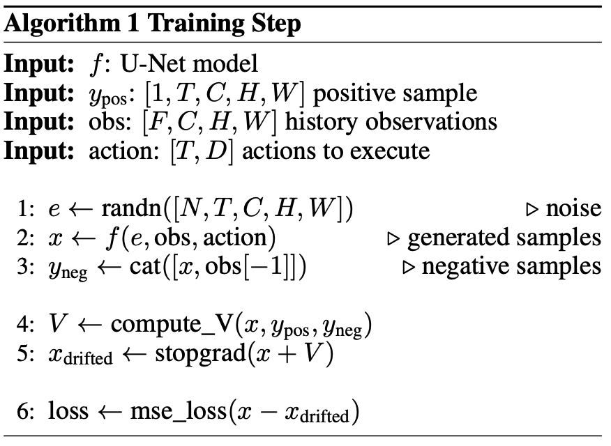
From the paper:

When training on a batch of $B$ videos, we perform this step (Algorithm 1) independently for each video. Since every video contains a unique sequence of history observations and actions, the model must compute $B$ distinct independent conditional drifting fields. Within each of these $B$ fields, the drift is calculated using a single positive sample (the ground-truth future frames) and $N_\text{neg}$ negative samples (the model's generated future frames). The total loss is the sum of the $B$ individual losses in the batch.

• 🔑 Walking through these steps in more detail: Suppose the batch contains $B$ different training videos.

0. Batch element $b$ has its own condition: $$c_b = \left(o_{t-F:t}^{(b)}, a_{t: t+T-1}^{(b)}\right), \quad b \in [1, B]$$and one ground-truth feature $y_b^+$, $N_{\text{neg}}$ generated futures $x_{b,1}, \ldots, x_{b, N_\text{neg}}$.
1. Because different videos generally have different scenes, histories, actions, and correct futures, the field for video $b$ is constructed only from: $$\{y_b^+, x_{b,q}, \ldots, x_{b, N_\text{neg}}, o_t\}$$It does not use the positive or generated samples belonging to another batch element $b'$. So at the broadest level: $$V^{(b)} = V_{p(\cdot \mid c_b), q_\theta(\cdot \mid c_b)}$$
2. Then the full batch contains: $V^{(1)}, V^{(2)}, \ldots, V^{(B)}$ → these are the aforementioned "$B$ distinct, independent conditional drifting fields."
   • Independent in the sense that $V^{(b)}$ only uses samples conditioned on $c_b$.

• ❓ Why must the drifting fields be separate?
  • Imagine batch element 1 is $c_1$ = "kitchen scene, move gripper right" and batch element 2 is $c_2$ = "table scene, move gripper left"
  • 💡 It would make no sense for particle $x_{1, i}$ generated for the first scene to be attracted toward the ground-truth future $y_2^+$ from the second scene.
  • 🔖 So the drift for condition 1 uses: $y_1^+, x_{1, 1}, \ldots, x_{1,N}$ and the drift for condition 2 uses: $y_2^+, x_{2, 1}, \ldots, x_{2, N}$ → that is conditional drifting!
• ❓ How does this fit with our analysis in Section #Feature space drifting?
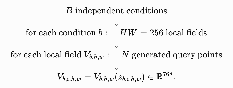
• 🔑 Note that one conditional vector field is a collection of local feature-space fields: $$V^{(b)} = \{V_{b, h, w}\}^{H,W}_{h=1, w=1} \implies \boxed{\text{one condition-level field} = \text{a grid of local feature-space fields}}$$

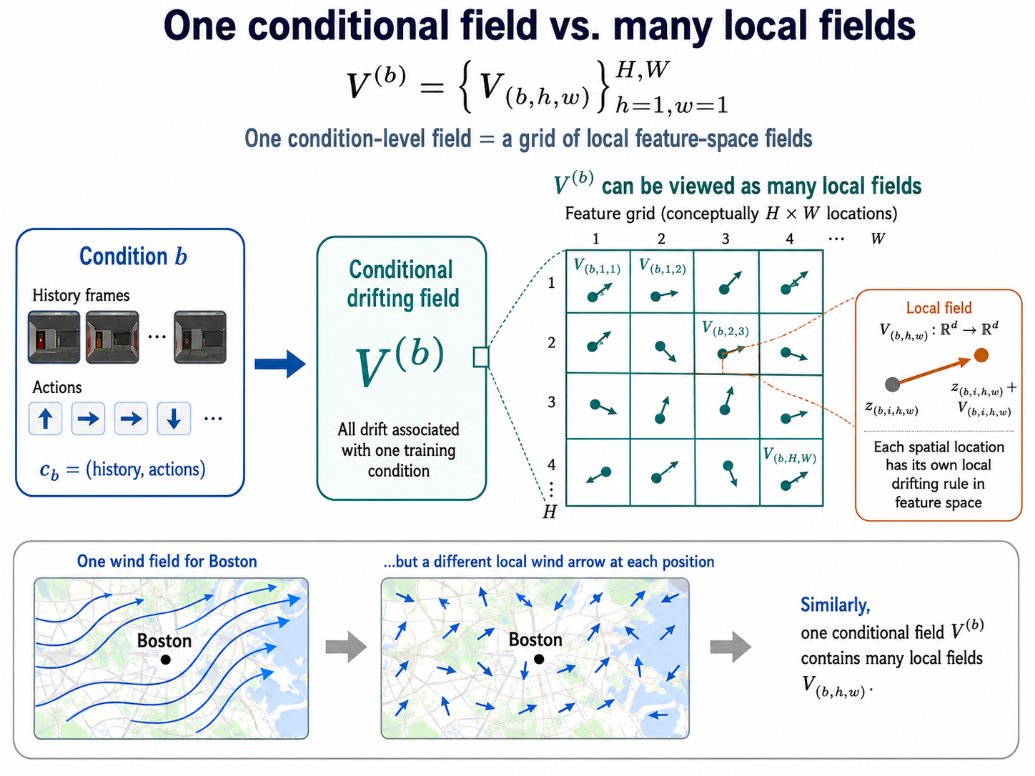
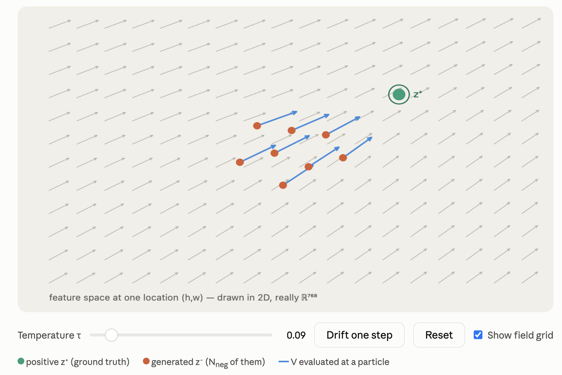
Normalization

To ensure that the drifting field is insensitive to the raw magnitudes and dimensionalities of samples in the feature spaces, the paper applies two normalizations:

1. Feature normalization so that the kernel takes on a reasonable range of values regardless of the samples' dimensionality
   • Divide samples by their average pairwise distance
   • Then compute the kernel as: $$k(x,y) = \exp \left(-\frac{1}{\tau \sqrt{C}}||\tilde{x} - \tilde{y}|| \right)$$
2. Normalize the drifting field by its magnitude so that multiple drifting fields can be summed together

Multi-temperature aggregation

After applying normalizations (#Normalization), they aggregate the drifting field across multiple kernel temperatures $\tau$: $$\tilde{V} = \sum_\tau \tilde{V}_\tau$$

Motion weighting

[Read into more.]

Feature extractor

On real-robot datasets, they compute the drifting loss in (i) the feature space of DINOv3 and (ii) the VAE latent space. The total loss is formed by summing these two components.

• DINOv3: $16 \times 16$ grid of $768$-dim. tokens, so we compute $256$ separate drifting losses on each of the spatial locations and take their weighted mean to form the overall DINOv3 drifting loss
• VAE-latent: $32 \times 32$ grid of $16$-dim. tokens, so we compute $1024$ separate drifting losses on each of the spatial locations and take their weighted mean to form the overall latent drifting loss

Self-forcing

Model training of DriftWorld occurs in 2 stages:

1. Condition DriftWorld on the ground-truth history frames
2. Initialize from stage 1 checkpoint^ and train by letting DriftWorld generate autoregressively, taking its own generated frames (with gradient detached) as input. Each of the $n_\text{neg}$ generated negative samples continues its own rollout.

Post-training on on failure demonstrations

For the Robomimic Lift and Can tasks, DriftWorld is initially trained on the multi-human dataset, which contains only successful demonstrations → i.e. the model is trained on a biased distribution with overly optimistic estimates of policy success.

• 🔑 They post-train the models (DriftWorld + baselines) on a dataset with a large percentage of failure demonstrations, which is created by rolling out early checkpoints of a diffusion policy.
• This enables the models to accurately simulate failures (since a good world model should simulate what actually would happen, which can consist of success and failure).

Data