Parametric types

• Bit#(n) := n-bit value
  • n is the parameter (an Integer value)
• Minispec provides other parametric types & you can define your own
  • Parametric types are generic
  • They take 1+ parameters
  • Parameters must be known at compile-time
  • Specifying the parameters yields a concrete type
• Parameters can be Integers or types
  • e.g. Vector#(n, T) is an n-element vector of T's

Integer is a special type

• Integer values (positive or negative) numbers with an unbounded number of bits
  • Unbounded bits → cannot be synthesized by hardware
• Integers are evaluated at compile time (turned into fixed numbers)
• Integer supports the same operations as Bit#(n): arithmetic, logical, comparisons, ...
  • 📍 Integer operations are evaluated by the compiler → operations on Integers never produce any hardware
  • Note: the compiler that does the integer operations is itself a piece of hardware that has the actual circuits used for computing integer operations. What we're highlighting here is the hardware circuit being generated by the compiler no longer contains the hardware for doing integer operations.

Parametric functions

• We can write one generic function that covers every case: e.g. rca#(n) builds a generic n-bit ripple carry adder
• 📍 Say you call a function in your HDL code. At compile time, the compiler will search for a matching concrete function, then fallback to the parametric function list and plug in the provided concrete values, then fallback to throwing errors.

Example: Parametric parity

$$\text{parity}(x) = x[0] \oplus x[1] \oplus \cdots \oplus x[n-1]$$where $\oplus$ := XOR.

• 💡 XOR of all the bits in $x$ gives us parity($x$) because it comes out to 1 when we have an odd number of 1s and 0 when we have an even number of 1s.

$$\text{parity}(x) = \text{parity}(x[n-2:0]) \oplus x[n-1]$$

• 🔖 In hardware languages, we usually have the most significant bit on the left and the least significant bit on the right (similar to binary) → hence x[n-2:0] instead of x[0:n-2] (latter being what Python does)

function Bit#(1) parity#(Integer n)(Bit#(n) x);
	return (n == 1)? x : x[n-1] ^ parity#(n-1)(x[n-2:0]);
endfunction

• ^ in English:
  • If only one bit, return the bit.
  • Else, use the recursive relation $\text{parity}(x) = \text{parity}(x[n-2:0]) \oplus x[n-1]$
• 🔑 Notes about the parametric function:
  • The parameter n is used as a variable in the function
  • Large circuits implemented by composing smaller ones: parity#(n) invokes parity#(n-1)
• If another function calls parity#(3), compiler produces:

// compiler realizes we need parity#(3), generates:
function Bit#(1) parity#(3)(Bit#(3) x);
	return x[2] ^ parity#(2)(x[1:0]);
endfunction
// compiler realizes we need parity#(2), generates:
function Bit#(1) parity#(2)(Bit#(2) x);
	return x[1] ^ parity#(1)(x[0:0]);
endfunction
// compiler realizes we need parity#(1), generates:
function Bit#(1) parity#(1)(Bit#(1) x);
	return x;
endfunction
// done :)!

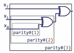
• ❓ Is this just recursion?
  • Recursion := you call a function inside of itself
  • ⚠️ In HDL, we never have recursion!
    • You cannot instantiate a circuit to do recursion by calling itself: module instantiation in hardware isn't a call, it's a physical copy.
    • Compile time vs. run time:
      • In most software, when you are doing recursion, you are doing it at runtime: you don't know how many times the function will call itself until it finishes running.
      • In hardware, you know concretely before runtime how many times the function will call itself - we recursively generate hardware code, but we are not recursively running it.
        • e.g. in function parity#(3) we call function parity#(2) which calls function parity#(1) → the functions are not calling itself!

N-bit ripple-carry adder

Let's work on building an N-bit RCA from the tree method (composing RCA2 → RCA4 → RCA8 → ...)!

function Bit#(n+1) rca#(Integer n)(Bit#(n) a, Bit#(n) b, Bit#(1) cin);
	Bit#(n/2 + 1) lower = rca#(n/2)(a[n/2-1:0], b[n/2-1:0], cin)
	Bit#(n-n/2 + 1) upper = rca#(n-n/2)(a[n-1:n/2], b[n-1:n/2], lower[n/2]);
	return {upper, lower[n/2-1:0]};
endfunction
// base case: rca#(1)
function Bit#(2) rca#(1)(Bit#(1) b, Bit#(1) cin);
	return fullAdder(a, b, cin);
endfunction
// ^in this way we give the n-bit rca function a base case without declaring a conditional within the n-bit function!

• Function header: function Bit#(n+1) rca#(Integer n)(Bit#(n) a, Bit#(n) b, Bit#(1) cin); = define a function called rca, parameterized by an integer n, that takes two n-bit inputs a and b plus a 1-bit carry-in cin and returns an (n+1)-bit result.
• Note: when n is an Integer, / behaves like integer division (i.e. equiv to //)
• 🔑 Indexing pattern to remember: a[j:i] = bits j, j-1, ..., i
  • Indexing in hardware is inclusive on both ends!
• 💡 In hardware, calling functions does not add any overhead in the way that it does in software:
  • In software, a function call is a runtime jump to some separate piece of code
  • In hardware, a function call is a blueprint for wiring → so whether we write the HDL by directly wiring together two pieces or call a function to do the wiring, we get the same circuit at runtime

Writing better Minispec code

Type inference

• You can omit the type of a variable by declaring it with the let keyword

Bit#(4) x = 4'b0011;
let y = x; // y has type Bit#(4)
let z = {x, x}; // z has type Bit#(8)
let w = 2'b11; // w has type Bit#(2)
let n = 42; // n has type Integer

User-defined types

• Type synonyms allow giving a different name to a type
  • e.g. typedef Bit#(8) Byte;
• Structs represent a group of member values with different types:

typedef struct {
	Byte red;
	Byte green;
	Byte blue;
} Pixel;

Pixel p;
p.red = 255;

• Enums represent a set of symbolic constants

typedef enum{
	Ready, Busy, Error
} State;
State state = Ready;

For loops

• For loop statements allow compactly expressing a sequence of similar statements

Bit#(6) w = 0;
for (Integer i = 0; i < 6; i = i + 1)
	w[i] = z[i / 2];

• ⚠️ For loops are not like loops in software programming languages:
  • Fixed number of iterations
  • Unrolled at compile time

Example: N-bit ripple-carry adder with loop:

function Bit#(n+1) rca#(Integer n)(Bit#(n) a, Bit#(n) b, Bit#(1) cin);
	Bit#(n) s = 0; // auto initializes to nx0s
	Bit#(n+1) c = {0, cin}; // auto concatenates enough 0s
	for (Integer i = 0; i < n; i = i + 1) begin
		let x = fullAdder(a[i], b[i], c[i]);
		s[i] = x[0];
		c[i+1] = x[1]
	end
	return {c[n], s};
endfunction

Conditionals

• Unlike software, both sides of every conditional are built into the circuit and computed at execution: we just choose between the outputs using a mux

A mux (multiplexer) is basically a tiny electronic selector switch.

Conditionals in HDL are not conditional execution: they connect two combinational circuits using a mux.

Design tradeoffs in combinational circuits

Algorithmic tradeoffs in hardware design

• Each function allows many implementations with widely different delay, area, and power
  • Lots of problems involve a tradeoff between area and time
• Choosing the right algorithms is key to optimizing your design
  • Let's build a better adder!

Better ripple-carry adder

Core idea: rca is slow because each bit may have to wait for the carry from the bit before it → sequential!

To compute the final answer of n-bit addition, rca requires the carry from the first bit to propagate all the way through every full-adder in order to finish. If we let $t_{PD}$ (PD := propagation delay) stand for the time we have to wait after changing an input before the circuit's output is guaranteed to have settled to the correct answer, rca takes $$t_{PD} = n\cdot t_{PD, FA} \in \Theta(n)$$amount of time to compute an n-bit add, where $n$ = number of bits in the adder, $t_{PD, FA}$ = propagation delay through one full adder, and $t_{PD}$ = worst-case propagation delay through the full rca.

Recalling runtime symbols:

• $O(n)$: no worse than linear
• $\Omega (n)$: no better than linear
• $\Theta(n)$: actually linear, up to constant factors.

• 🔖 So, rca scales linearly with input size.

How do we make adding faster?

Carry-select adder

We can trade area for speed using a carry-select adder!

• 💡 Compute two copies of the upper half of the adder: one assumes cin=0, the other assumes cin=1. Then, compute these two routes + the lower half of the adder in parallel, and use a mux to select with upper half adder's results to use after the lower half is done computing.

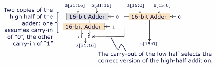
• We can recursively apply this idea to each n/2-bit adder, which yields: $$t_{PD, n} = \Theta(\log n)$$

Carry-lookahead adder (CLAs)

• CLAs compute all carry bits in $\Theta(\log n)$ delay with low area overhead

Appendix

When writing HDL, you should realize that the code you write directly translates to the physical world! So passing in a parameter of 64 to an N-bit rca function will create lots of physical gates.

Combinational logic vs. sequential logic

Combinational circuit

A combinational circuit is like a machine made of pipes and valves where water flows in one direction only. Whatever you pour in the top comes out the bottom, transformed, and the output depends only on what you are pouring in right now. The machine has no memory.

Formally, a combinational circuit is a directed acyclic graph of gates. Each gate's output is a Boolean function of its inputs, and because there are no cycles, you can topologically sort the gates and evaluate them in order.

• 💡 The output of a combinational circuit is therefore a pure function on the current inputs: $y = f(x)$, with no dependence on history.
• 🔖 Examples:
  • Adders, multiplexers, decoders, parity XOR tree, an ALU
• 📍 Recursion is not possible in combinational circuits, because it requires applying the same function to its own output (a loop)
  • With acyclicity, the only way to apply $f$ to its own output is to build a second physical copy of $f$ downstream.
• ⚠️ Example of a problematic loop: inverters!

Sequential circuit

A sequential circuit adds buckets: you can pour water in, hold it in a bucket, and then on the next tick empty the bucket into the pipes again. The machine remembers what it did last time.

We'll learn more about this in following lectures!

• 💡 Central idea:
  • Combinational circuits pay for implementing loops using space
  • Sequential circuits pay for implementing loops using time